The thing started my wife ask me how to understand the 3-dimension object created by the array() function in R. We know that if there are only 2 dimensions, they are the x-axis and y-axis in a plot. And in R (or any other terminal tool), it looks like rows and columns. For example, below I created a 2-dimension array data. (In most case, I always call them matrix or data.frame, maybe I have been wrong for a very long time...haha)
> d2 <- array(1:(4 * 5), c(4,5))
> d2
     [,1] [,2] [,3] [,4] [,5]
[1,]    1    5    9   13   17
[2,]    2    6   10   14   18
[3,]    3    7   11   15   19
[4,]    4    8   12   16   20
Other functions like matrix(), data.frame() .etc can reach similar results. In short, in the above example, we get a 2-dimension data structure with rows and columns. Then as we know, the apply() function is a very nice way to quickly iterate rows or columns.
> test <- apply(d2, 1, function(x) print(x))
[1]  1  5  9 13 17
[1]  2  6 10 14 18
[1]  3  7 11 15 19
[1]  4  8 12 16 20
>
> test <- apply(d2, 2, function(x) print(x))
[1] 1 2 3 4
[1] 5 6 7 8
[1]  9 10 11 12
[1] 13 14 15 16
[1] 17 18 19 20
>
Then here comes the important part. I know many people are "memorying" that the second parameter in the apply() function decided the dimension it iterates, including me before. So we all think that 1 indicates rows, and 2 indicates columns right? So there come two vital questions:
- How the second parameter works for multi-dimension arrays? If you have 3 dimensions, then what the "first" dimension (1) iteration result will be?
- What will
apply(d2, c(1,2), function(x) print(x))output?
Visualisation of 3-Dimension Array
So I want to visualise the 3-Dimension array a bit. I firstly created a 3D array here. I defined a 3D array with 3 dimensions as 2, 3, 4 separately. The purposed is if dimensions have different value, it's easier for me to find which one is which.
d3 <- array(1:c(2 * 3 * 4), c(2, 3, 4))Then let's have a look at what it looks like below. Seems we can see there are 4 matrixes, that there is a ,,1 at the beginning of each, so we can guess out that the ,, indicates 3 dimensions, and ,,[], the third value after the second comma indicates the third dimension. There are 4 matrixes here because previous I defined the three dimensions as c(2, 3, 4). Only the third dimension has 4 elements. The first dimension should only have 2 elements, while the second dimension should only have 3 elements.
> d3
, , 1

     [,1] [,2] [,3]
[1,]    1    3    5
[2,]    2    4    6

, , 2

     [,1] [,2] [,3]
[1,]    7    9   11
[2,]    8   10   12

, , 3

     [,1] [,2] [,3]
[1,]   13   15   17
[2,]   14   16   18

, , 4

     [,1] [,2] [,3]
[1,]   19   21   23
[2,]   20   22   24

>
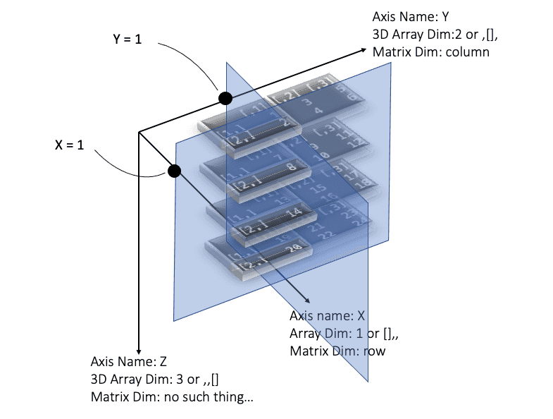
Above is still hard for us to understand the 3D structure of the data. And even, later we want to see how the apply() function works on it. So I decided to visualise it. In the below figure, I just screenshot the above 4 matrixes, then rotated a bit via Powerpoint. Now we can clearly see the 3 dimensions. In the above plot there are 3 axes, normally in 2-dimension matrixes, we normally only can see two axes (X and Y), we named them as row and column in 2-dimension. However, in the 3D situation, we need to add one more axis (I named it as Z here), which does NOT exist in the 2D situation. That's why I can't simply call it "hight" or "tall" or anything.
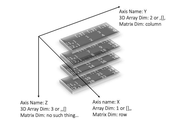
One very interesting thing is, I think in the above figure, the 3 dimensions actually have many names in different scenarios. For example, as I labelled in the above plot, name X, Y, and Z are named by me, which means maybe for other people, they prefer to think the Y axis in my plot should be labelled as X. These names are mathematical or even just personal labels, it varies.
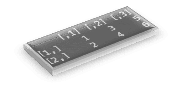
However, in R language, it has defined the three dimensions, which is fixed and not changeable by personal ideas. For example, my above plot shows, the third dimension (Z axis) is the one vertical to the floor. So it means if you are selecting a 3D array by the third dimensions (Z axis). You are actually selecting a horizontal slice through the 3D objects.
> d3[,,1]
One Dimension Selection with a 3D array
It's so common in R that we need to select certain rows or certain columns when we working on a 2-D matrix. In the above example, we have shown that if things turn to 3D, it's harder for us to select just via one dimension: It actually selects a plate, or in another word, a slice of a 2D matrix. Here I will give more examples.
So now we can infer, if we now use the apply() function here as the third dimensions, it will cut all data horizontally into 4 slices, then iterate each matrix.
> test <- apply(d3, c(3), function(x) print(x))
     [,1] [,2] [,3]
[1,]    1    3    5
[2,]    2    4    6
     [,1] [,2] [,3]
[1,]    7    9   11
[2,]    8   10   12
     [,1] [,2] [,3]
[1,]   13   15   17
[2,]   14   16   18
     [,1] [,2] [,3]
[1,]   19   21   23
[2,]   20   22   24
>
Now we know how and what exactly the third (Z) axis is, and how can we iterate it via a loop. So what d3[1,,] return? By checking the plot, we can infer that we can get another slice, but not horizontally, but vertically and parallel to the wall created by the Y and Z-axis. Like below, when we run d3[1,,], we are setting X-axis as 1, while no restriction for the Y or Z axis. So it can be seen as a vertical slice plate that was cut through X-axis but parallels with the wall created by the Y and Z axes. So eventually we can get a 2-dimension matrix on that vertical slice.
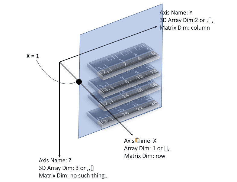
> d3[1,,]
     [,1] [,2] [,3] [,4]
[1,]    1    7   13   19
[2,]    3    9   15   21
[3,]    5   11   17   23
>
The same logic could work for Y-axis. If we select d3[,1,], you can imagine we are selecting a slice plate parallel to the wall created by the X and Z axis. And it will return a 2-d matrix:
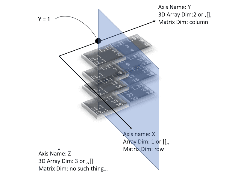
> d3[,1,]
     [,1] [,2] [,3] [,4]
[1,]    1    7   13   19
[2,]    2    8   14   20
>
Have you considered, why when we select d3[,1,], it returns as above matrix instead of:
     [,1] [,2]
[1,]    1    2
[2,]    7    8
[3,]   13   14
[4,]   19   20
The above matrix seems more obvious from my figure, why there is rotation here? My understanding is there is a ranking priority between the 3 dimensions. The X-axis has the highest priority, so if X-axis exist, which means we are selecting the X-axis, the returned matrix will take the X-axis as rows and the other axis as columns. Thus in my above example, then Y=1, the X-axis (contains 2 values) will be set rows and Z-axis (contains 4 values) will be set as columns. So eventually a 2 by 4 matrix is returned. If X-axis does not exist, say d3[1,,], Y-axis have a higher priority over the Z-axis, it will return Y-axis as a row, and Z axis as columns.
In short, for me, it's not easy to select even one dimension from a 3D array.
- It's more like cutting slices into a 3D object and get pieces of plates from them.
- The returned matrix may be rotated based on priorities of different dimensions.
- It's hard to match names between them. Make sure you have correctly matched them every time you are using the 3D array.
- 1): The second parameter
c(1,2,3)inapply(); - 2):
d3[*,*,*]in raw R code; - 3): Names like row, column, other like higher.
- 4): Other common names like X/Y/Z axis.
- 1): The second parameter
All these cause potential programming bugs for analyser.
Two Dimension Selection with a 3D array
Then we can have a look how to select 2 Dimensions togather from 3D array. In other word, what code like apply(d3, c(1,2) function(x) print(x)) would retrun? When we use apply() function, it will create a index list based on our parameter setting. When we set the second parameter as c(1), it will return: d3[1,,], d3[2,,] . So if we set the parameter as c(1,2). It will return:
d3[1,1,], d3[2,1,], d3[1,2,], d3[2,2,], d3[1,3,], d3[2,3,]As you can see, it's just the combination of the first (x) and second (y) dimensions, There are only 2 values in the first dimensions, and there are only 3 values in the second dimensions, so there are a totally 2*3=6 combinations. Then the apply() function will fetch data based on these 2-D index one by one, and iterate the whole data. Now, what would be returned if both X and Y axis are selected? Yes, a vector across Z-axis. You can image a drill into the 3D object. Below I draw an example of d3[2,1,]:
The code is below:
> test <- apply(d3, c(1,2), function(x) print(x))
[1]  1  7 13 19
[1]  2  8 14 20 # Above plot shows this one: X=2 & Y=1
[1]  3  9 15 21
[1]  4 10 16 22
[1]  5 11 17 23
[1]  6 12 18 24
>
An example to use a 3D array?
In the above sample, I show what would happen if you directly created 3D array with pure numbers. The result is you get a complex and hard to read/understand/work data structure. I never used multiple dimensions array in my work, merely because I think it would be super easy to make mistake in coding. However, after some thinking, I think if the data structure is representing a certain level of real-world thing, multiple-array may be a good idea. Below is an example I did, I downloaded GDP per sector for per England regions and per year from official GOV website.
So the excel I downloaded contains UK's each regions' GDP per sectors like Agriculture, Mining .etc in each year from 2012-2019. So I will try to read the data into R and form a 3D array. I read them all into a list, then use unlist function to collapse them all into a long vector. Then finally created a 3D array from the long vector. Note that the dimnames parameter is highly recommended to name the x/y/z axis. Finally, I get the 3D array object UKRegionGDPbyYear.
library("readxl")

RegionName <- as.data.frame(read_excel("./rgdptables19q430072020113950.xlsx", sheet=1, skip=8, n_max=11, col_names=FALSE))[,1]
SectorName <- as.character(as.data.frame(read_excel("./rgdptables19q430072020113950.xlsx", sheet=3, skip=4, n_max=1, col_names=FALSE))[1,2:23])
SectorName <- sapply(SectorName, function(x) strsplit(x, split=",")[[1]][1])
Years <- as.character(c(2012:2019))

GDP <- list()
for(i in 3:13)
{
    tmp <- as.data.frame(read_excel("./rgdptables19q430072020113950.xlsx",sheet=i, skip=8, n_max=8, col_names=FALSE))[,3:24]
    rownames(tmp) <- Years
    colnames(tmp) <- SectorName

    GDP[[RegionName[i-2]]] <- tmp
}

UKRegionGDPbyYear <- array(unlist(GDP),
                           c(length(Years), length(SectorName), length(RegionName)),
                           dimnames = list(Years, SectorName, RegionName)) # The dimnames is recommanded here.
In the final UKRegionGDPbyYear object, the first dimension is Years, the second dimension is Sectors, and the third dimension is RegionName. Thus since we know their real-world meanings, we can easily select data we want like, answer questions like:
- What is the "Education" sector's GDP in each England region per year?
> UKRegionGDPbyYear[,"Education",]
     North East North West Yorkshire and The Humber East Midlands West Midlands
2012       99.5       94.3                     92.6         102.2         100.6
2013       98.3       98.4                     96.6         103.2         100.1
2014       96.5       97.1                     99.1         102.9          99.9
2015       97.1       98.7                    102.7         101.9         100.4
2016      100.0      100.0                    100.0         100.0         100.0
2017       96.1      102.6                     98.7         104.5         103.6
2018       94.1      102.9                    101.0         104.8         108.1
2019       86.2      105.3                    100.8         113.6         101.3
     East of England London South East South West England Wales
2012           102.3   98.8       94.0       94.4    97.2 100.1
2013           102.5   98.7       96.7       96.8    98.7 102.0
2014            98.2  103.2       95.6       97.8    99.2  99.3
2015            98.1  105.4       98.3       97.6   100.6  99.7
2016           100.0  100.0      100.0      100.0   100.0 100.0
2017            99.9  102.8      100.9       99.4   101.4  98.3
2018           103.4  104.6       98.8       98.0   102.2  95.1
2019 111.2 113.4 103.5 98.5 105.7 100.6- What is London's GDP in the "Arts" sector in 2012-2015 ?
> UKRegionGDPbyYear[c("2012","2013","2014","2015"),"Arts","London"]
2012 2013 2014 2015
89.4 88.5 93.3 99.0
>- What is London's top 5 GDP sector in 2019?
> sort(UKRegionGDPbyYear["2019",,"London"],decreasing=TRUE)[1:5]
                                            Mining & quarrying
                                                         168.5
                                 Information and Communication
                                                         122.2
                 Administrative and support service activities
                                                         118.4
Wholesale and retail: repair of motor vehicles and motorcycles
                                                         116.7
                                                   Agriculture
                                                         114.9
>
In short, when you create a multiple dimension array with some real-world thing represented (and named in dimensions). It would be easier to use.